Create the Blue Book for Bulldozers Model
Jupyter Notebooks
The following is an excerpt from a live session dedicated to reviewing the Jupyter Notebook that makes up the solution for this particular Kaggle Competition Example.
After watching this video you will deploy a Notebook Server where you will use a Jupyter Notebook to create a model for Blue Book for Bulldozers.
(Hands-On) Create a Notebook in Your Kubeflow Cluster
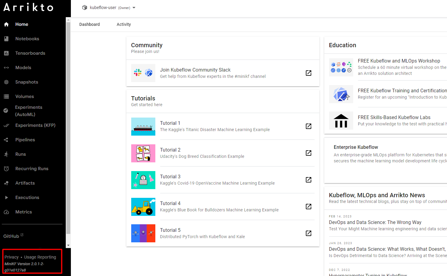
1. Check your Kubeflow version
To check your version, refer to the bottom left corner in the Central Dashboard:
Remember your Enterprise Kubeflow version, as you will need to follow instructions that are specific to the version you are running.
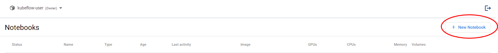
2. Navigate to Notebooks
Navigate to the Notebooks tab on the Enterprise Kubeflow Central Dashboard:

3. Create a new notebook
Click on + New Notebook.
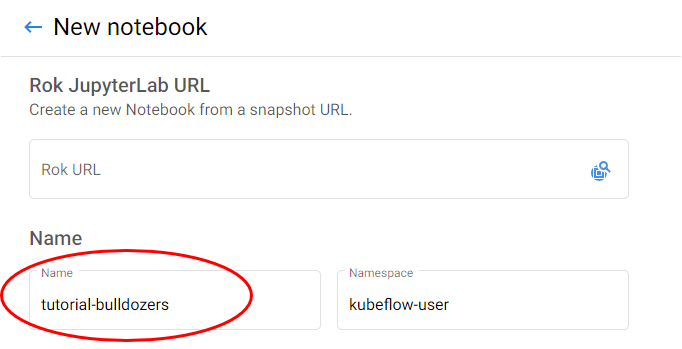
4. Name your notebook
Specify a name for your notebook.
5. Select Docker image
Make sure you are using the default Docker image. This image will have the following naming scheme:
gcr.io/arrikto/jupyter-kale-py38:<IMAGE_TAG>
gcr.io/arrikto/jupyter-kale-py36:<IMAGE_TAG>
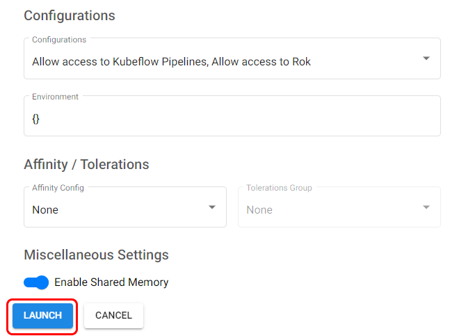
6. Create your notebook
Click LAUNCH to create the notebook.
7. Connect to your notebook
When the notebook is available, click CONNECT to connect to it.

(Hands-On) Download the Data and the Notebook into Notebook Server
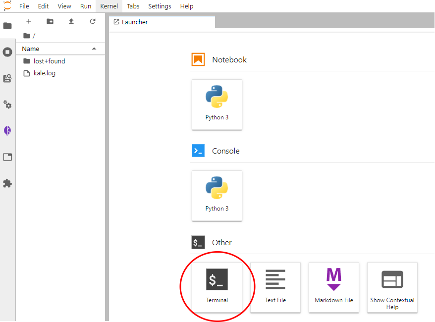
1. Open a new terminal
A new tab will open up with the JupyterLab landing page. Create a new terminal in JupyterLab:
2. Download the notebook and data
Run the following command in the terminal window to download the notebook file and the data that you will use for the remainder of this course. Choose one of the following options based on your version:
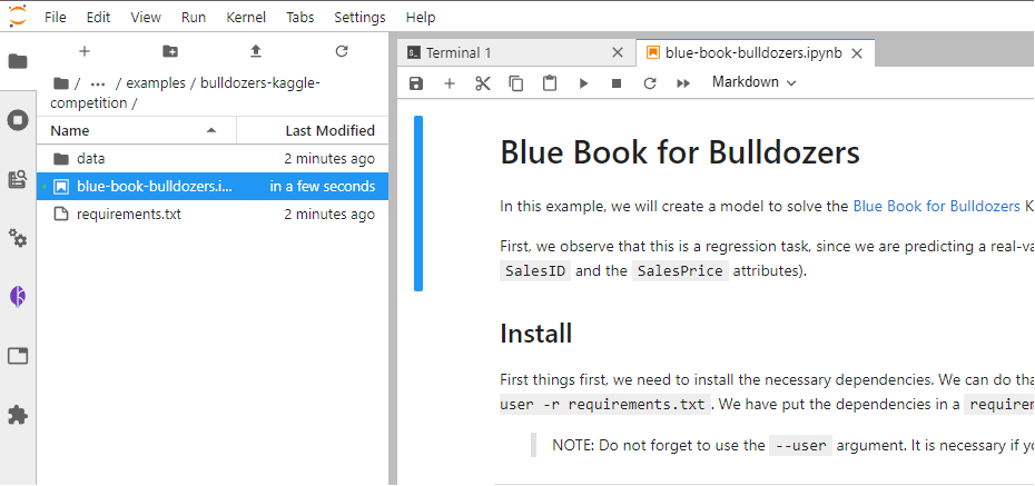
git clone https://github.com/arrikto/examplesgit clone -b release-1.5 https://github.com/arrikto/examples3. Open the Notebook
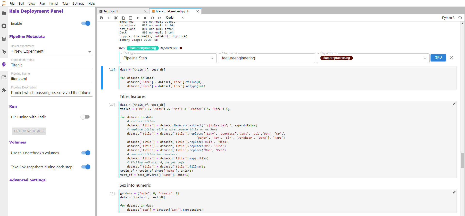
This repository contains a series of curated examples with data and annotated notebooks. Navigate to the folder examples/academy/bulldozers-kaggle-competition/ in the sidebar and open the notebook blue-book-bulldozers.ipynb
Compile and Run an AutoML Workflow from Notebook
(Hands-On) Install Packages and Libraries for Notebook
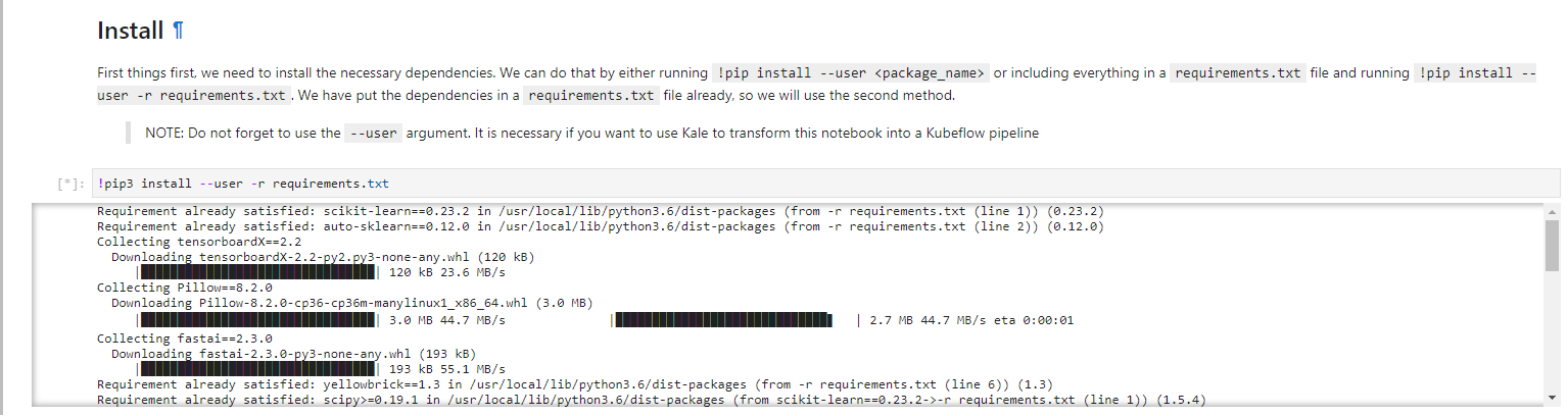
1. Install the necessary dependencies
Run the cell to install the necessary dependencies:
Normally, you should create a new Docker image to be able to run this notebook as a Kubeflow pipeline, to include the newly installed libraries. Fortunately, Rok and Kale make sure that any libraries you install during development will find their way to your pipeline, thanks to Rok’s snapshotting technology and Kale mounting those snapshotted volumes into the pipeline steps.
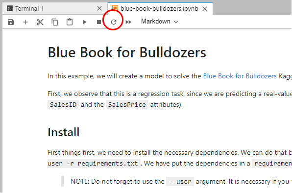
2. Restart the notebook kernel
Restart the notebook kernel by clicking on the Restart icon:
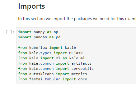
3. Run the imports cell
Run the imports cell to import all the necessary libraries:
(Hands-On) Load and Prepare Your Data
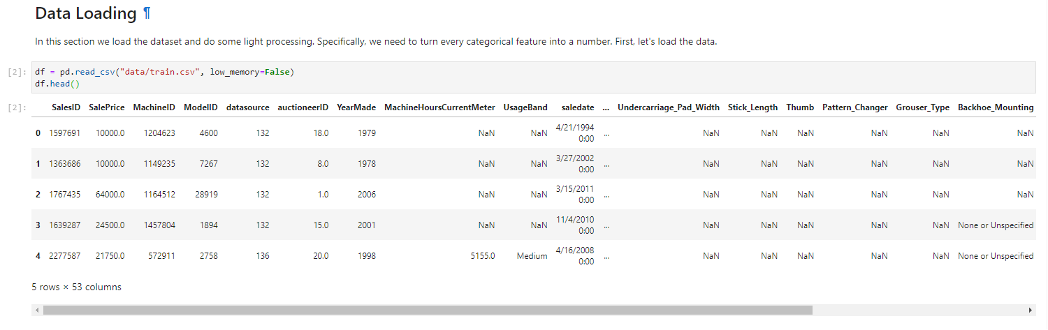
1. Load the dataset
Run the cell that loads the dataset:
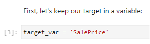
2. Keep the target value in a variable
Our target variable is SalePrice. Run the cell to keep it in a variable:
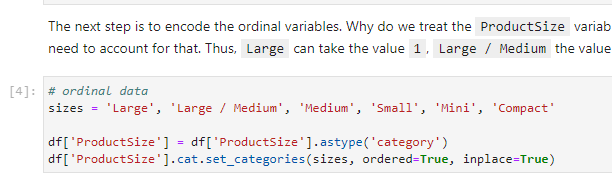
3. Encode the ordinal variables
Run the corresponding cell to encode ordinal variables:
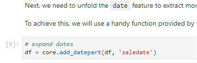
4. Unfold the dates
Run the cell to unfold the dates to engineer more features:
5. Split the dataset
Run the cell to split the dataset into train and valid sets:
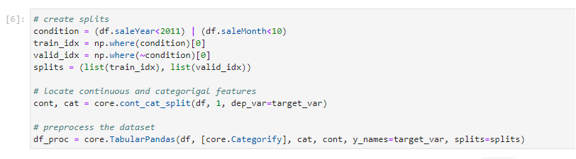
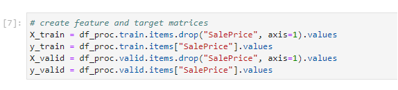
6. Extract features and labels
Run the cell to extract features and labels into numpy arrays:
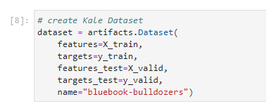
7. Group together the dataset
Run the cell to group together the dataset using the Kale Dataset
Pipeline Creation w/ Kale Overview
What is Kale JupyterLab Extension?
KALE (Kubeflow Automated pipeLines Engine) is a project that aims at simplifying the Data Science experience of deploying Kubeflow Pipelines workflows. Kale is built right into Kubeflow as a Service and provides a simple UI for defining Kubeflow Pipelines directly from your JupyterLab notebook. There is no need to change a single line of code, build and push container images, create KFP components, or write KFP DSL code to define the pipeline DAG.
With Kale, you annotate cells (which are logical groupings of code) inside your Jupyter Notebook with tags. These tags tell Kuebflow how to interpret the code contained in the cell, what dependencies exist, and what functionality is required to execute the cell.
To create a Kubeflow Pipeline (KFP) from a Jupyter Notebook using Kale, annotate the cells of your notebook selecting from six Kale cell types.
Imports
Are a block of code that imports the packages your project needs. Make it a habit to gather your imports in a single place.
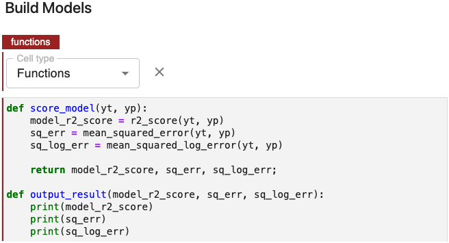
Functions
These represent functions or global variable definitions other than pipeline parameters to be used later in the machine learning pipeline. These can also include code that initializes lists, dictionaries, objects, and other values used throughout your pipeline. Kale prepends the code in every Functions cell to each Kubeflow Pipeline step.
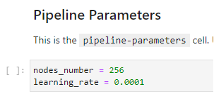
Pipeline Parameters
These are used to identify blocks of code that define hyperparameter variables that are used to finely tune models.
Pipeline Metrics
Kubeflow Pipelines supports the export of scalar metrics. You can write a list of metrics to a local file to describe the performance of the model. The pipeline agent uploads the local file as your run-time metrics. You can view the uploaded metrics as a visualization on the Runs page for a particular experiment in the Kubeflow Pipelines UI.
Pipeline Step
A step is an execution of one of the components in the pipeline. The relationship between a step and its component is one of instantiation, much like the relationship between a run and its pipeline. In a complex pipeline, components can execute multiple times in loops, or conditionally after resolving an if/else like clause in the pipeline code.
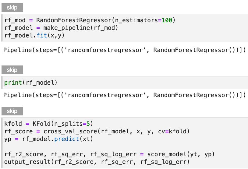
Skip Cell
Use Skip to annotate notebook cells that you want Kale to ignore as it defines a Kubeflow pipeline.
Now, we are ready to run our AutoML experiment using Kale.
(Hands-On) Start the AutoML Workflow Using Kale
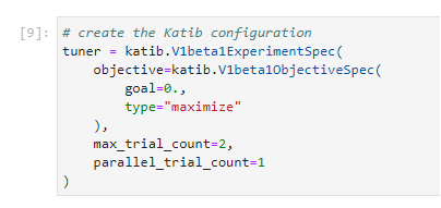
1. Create a Katib configuration
This step will ensure that after finding the best configuration, Kale will start a Katib experiment to further optimize the model. In the next section, you will find more information about how we use Katib to perform hyperparameter optimization on the best-performing configuration. Run the cell to create a Katib configuration:
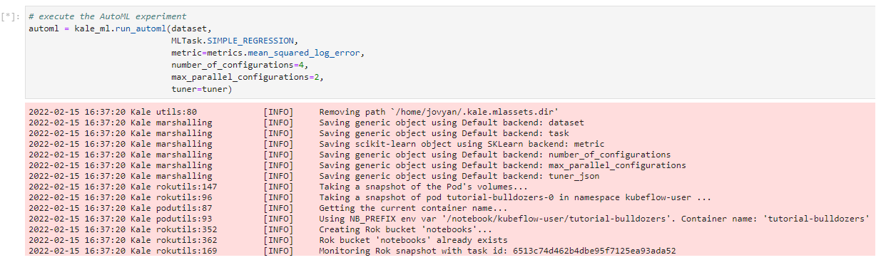
2. Run the AutoML experiment
Run the cell to run the AutoML experiment:
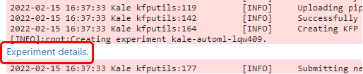
3. View the Kubeflow Pipelines (KFP) experiment
Kale creates a Kubeflow Pipelines (KFP) experiment. Click on Experiment details to view it:
This will open the experiments page:
4. View the Kubeflow Pipelines (KFP) pipeline
Kale creates a KFP pipeline that orchestrates the AutoML workflow. Click on Run details to view it:
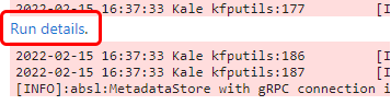
This will open the pipeline run page:
5. Monitor the experiment
You can monitor the experiment by printing a summary of the AutoML task at any point in time. This is how it will look like when all the runs have completed:
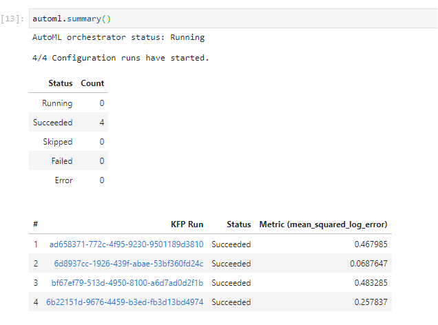
The whole AutoML workflow needs about 30 minutes to complete. You can continue with the next sections, but some steps or pipelines may still be in progress.
The Power of Kale
Kubeflow Pipelines components are based on the compiled data science code, pipeline step container images, and associated package dependencies.
A well-defined pipeline has the following characteristics.
- A quick way to give our code access to the data we want to use.
- An easy way to pass the data between steps.
- The flexibility to display outputs.
- The ability to revisit / reuse data without repeatedly querying external systems.
- The ability to opt-out of unnecessary steps that really were meant for experimental purposes.
- The confidence that our imports and function dependencies are addressed.
- The flexibility to define Hyperparameters and Pipeline Metrics within our Jupyter environment and store them within our pipeline definitions.
Consider the following steps that are eliminated by working with Kale and the time saved as well as the consistency introduced by eliminating these steps.
- Repetitive installation of Python packages: With Kale, all the necessary packages are installed at once.
- Slow pipeline creation: Toil intensive time to code the pipeline vs taking advantage of Kale’s pipeline automation capabilities.
- Lots of boilerplate code and code restructuring: Without Kale, the notebook has to be entirely modified to be compatible with the KFP SDK, which results in having to write more boilerplate code. With Kale, the original notebook is simply annotated with Kale tags.
- Pipeline visualization setup difficulty: To produce metrics visualization, specific standards and processes must be followed. With Kale, the visualizations are created in the same conventional way we create visualizations in our notebooks.
Kubeflow Pipelines give you the connective tissue to train models with various frameworks, iterate on them, and then eventually expose them for the purpose of serving. This means our entire Model Development Lifecycle lives within our KubeFlow pipeline components and definitions. We now have the power to be intentional and declarative with how we want our models to be developed as well as how we provide feedback loops to our data science teams. This gives us the capacity to further improve not only the data science function code but the pipeline descriptions themselves in order to respond to ever-growing business demands. This lays the foundation for the Continuous Integration and Continuous Deployment processes which ultimately push and support models in production. This can become quite daunting if you are taking the manual approach. What works for your organization today might suffer the technical debt-ridden test of time as you begin to scale and introduce essential complexity that comes from improved velocity and feature offerings. Your data engineering team should not need to scale linearly with your data scientists. Leveraging Kale means you are setting the foundation for an effective and self-sustainable MLOps culture and environment
If you would like to see how to do this without using Kale please read through the following blog post: https://www.arrikto.com/blog/developing-kubeflow-pipelines-kaggles-digit-recognizer-competition/. Keep in mind that your Pipeline must be structured in a way that the steps flow as necessary, likely some combination of in sequence and in parallel. This structuring also requires managing imports and package dependencies as well as how the intermediate data is moved across Pipeline Steps. This requires design forward-thinking to support and understand how you are going to move prepared data and work done by our components across your platform with the eventual goal of serving predictions from an inference server endpoint. Pipeline components (and what they consume) greatly impact the health of your model development life cycle. This is especially true with the data used for training, but can also refer to the ConfigMaps, Secrets, PersitentVolumes, and their respective PersistentVolumeClaims that are created within the context of the Pipeline. It’s important to understand what is truly immutable, and what can be changed or misunderstood. The easiest example is a data lake or a volume. A snapshot of the current state of these tools can drastically improve your reproducibility and allow you to regain your control over your MLOps outcomes with immutable datasets. For more technical detail on this specific topic please refer to the OSS Documentation: https://www.kubeflow.org/docs/components/pipelines/overview/quickstart/.
Also, keep in mind that during execution there are a myriad of supporting technical exercises that will have to be coded into any Pipeline that is created manually. You will need to marshal work done within a step to volumes so you can enhance your ability to move data between components and subsequent steps to ensure proper continuity in your pipeline. If you don’t have work from the previous steps or consolidate work run in parallel, you can create problems for tasks further down the line or submit degraded outputs for steps to consume. Once you properly align your inputs and outputs, you will also need to precompile the code, upload it to the Kubeflow Deployment and actually execute the Pipeline. This can be extra difficult if you want to ensure the SAME volumes are passed along during each run. New volumes can be provisioned and “bring less baggage”, but then you are potentially creating a “dead asset” that is not only taking up precious space but can also be a security risk. We also must consider the frequency of a run and what garbage collecting must be done from our recurring pipelines. This is even touching the volume access modes which means we need to not only provision a volume but make sure that whatever needs to reach the volume (independently or with other tools) CAN access the volume. This can be a lot to manage and lead to failed smoke tests leading to slower deployments or promotion failures. For ease of use and toil-free uptime, we strongly recommend working with Kale!
MLOps and Kubeflow Pipelines
Kubeflow Pipelines give you the connective tissue to train models with various frameworks, iterate on them, and then eventually expose them for the purpose of serving with Kserve. This means that once the work has been done in a Jupyter Notebook and the code converted to a Kubeflow Pipeline with Kale, the entire Model Development Lifecycle lives within the Kubeflow pipeline components and definitions. A well-defined pipeline has the following characteristics.
- A quick way to give code access to the necessary data.
- An easy way to pass the data between steps.
- The flexibility to display outputs.
- The ability to revisit / reuse data without repeatedly querying external systems.
- The ability to opt-out of unnecessary steps that are meant for experimental purposes.
- The confidence that imports and function dependencies are addressed.
- The flexibility to define Hyperparameters and Pipeline Metrics within the Jupyter environment and store them within pipeline definitions.
- Everything can be easily managed and consolidated within the notebook(s) to prevent juggling tabs, tools, and toil.
For more technical detail on this specific topic please refer to the OSS documentation: https://www.kubeflow.org/docs/components/pipelines/introduction.
The Kubeflow Pipelines that Data Scientists create with Kubeflow are both portable and composable allowing for easy migration from development to production. This is because Kubeflow Pipelines are defined by multiple pipeline components, referred to as steps, which are self-contained sets of executable user code. Kubeflow Pipelines components are based on the compiled data science code, pipeline step container images, and associated package dependencies. Each step in the pipeline runs decoupled in Pods that have the code and reference the output of previous steps. Each container (often acting as a base for a pipeline step) can be stored in a centralized Container Repository. Managing containers via the Container Registry introduces versioning and model lineage tracking for future audits and reproducibility needs. Snapshots are taken of the Kubeflow Pipeline at the start of execution, before and after each step in the pipeline. Ideally, in the future state, each training run produces a model which is stored in a Model Registry and execution artifacts that are stored in their respective Artifact Stores. As a result, the entire lineage of the model is preserved and the exact steps that are required to create the model in another environment can be shared. This lays the foundation for the Continuous Integration and Continuous Deployment processes which ultimately push and support models in production. We will discuss Continuous Integration and Continuous Deployment towards the end of this course.
(Hands-On) Obtain the Different Configurations
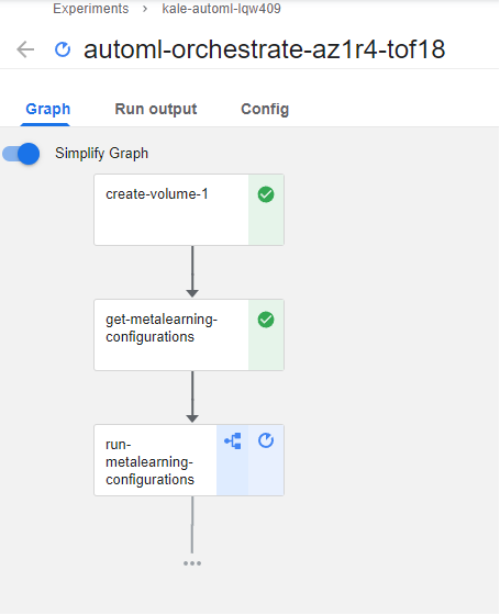
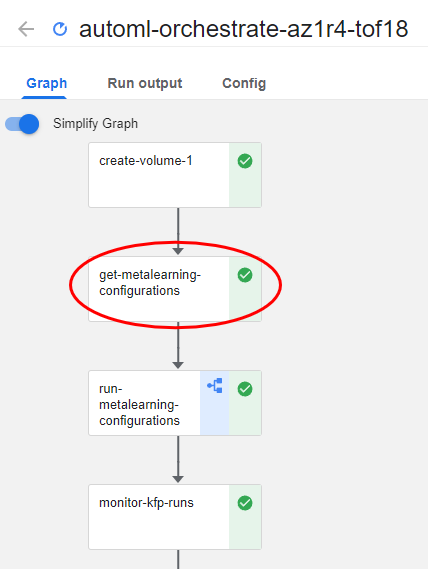
1. View the orchestration pipeline
Let’s take a look at the orchestration pipeline that Kale produced. During the get-metalearning-configurations step, Kale asks auto-sklearn to provide AutoML configurations. A configuration is an auto-sklearn “suggestion”, composed of a model architecture and a combination of model parameters that auto-sklearn thinks will perform well on the provided dataset.
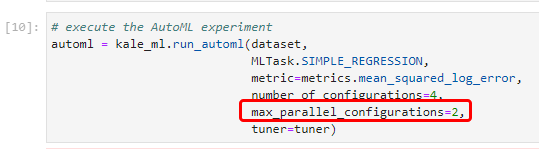
In this example, Kale asks from auto-sklearn to produce four different configurations. You defined this in a notebook cell previously as shown below:
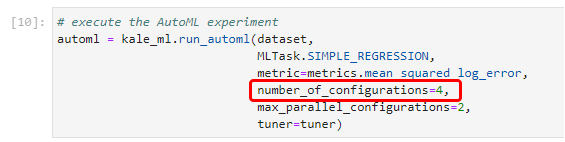
In a production environment, this number would be in the order of tens or hundreds. Kale would ask auto-sklearn to suggest many different configurations based on the provided task and dataset.
Note that some configurations could share the same model architecture, but different initialization parameters.
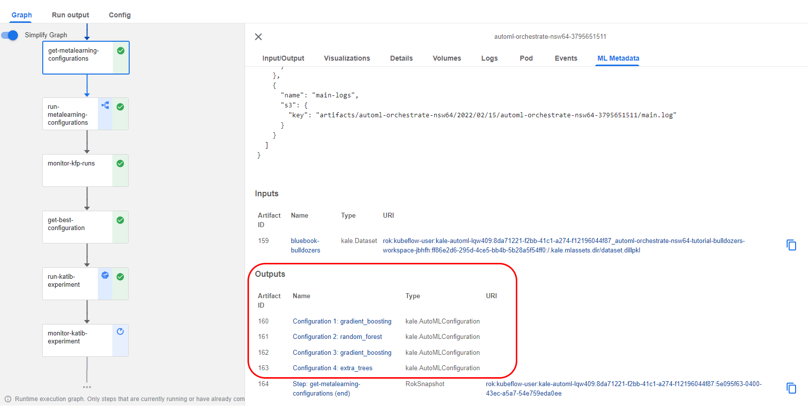
2. View the configurations
If you click the step and go to the ML Metadata tab, you will see the configurations that auto-sklearn produced:
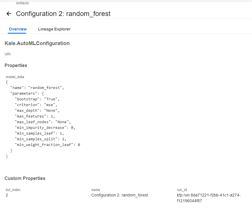
3. View the second configuration
Let’s click on the second configuration:

4. View the model and the initialization parameters
We can see the model and the initialization parameters:
(Hands-On) Create a KFP Run for Each Configuration
Auto-sklearn configurations are just an “empty” description of a model and its parameters. We need to actually instantiate these models and train them on our dataset.
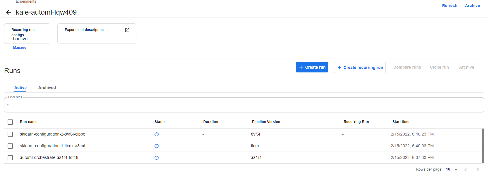
1. View the parallel runs
Kale will start a KFP run for each configuration, that is it will start four pipeline runs. By default, these KFP runs will execute in parallel, so this can become a massive task for your cluster. Here, we have configured Kale so that it starts just two runs simultaneously at any given point in time. We did this previously in the notebook:
Kale produces these KFP runs during the run-metalearning-configurations step:
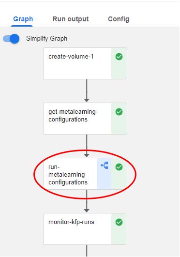
Notice the pipeline icon that this step has. This means that it produces one or more KFP runs.
2. Go to run-metalearning-configurations step
If you click on the step and go to the ML Metadata tab, you will find the four runs that Kale produces during this step (Kale will populate the metadata tab with these link at runtime, while it starts the runs):
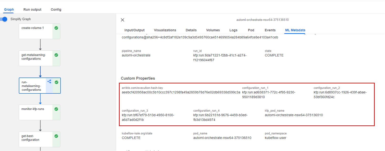
These pipelines look identical. They just train a different model and/or have different initialization parameters.
3. View a configuration KFP run
Let’s click one of them to view the KFP run:
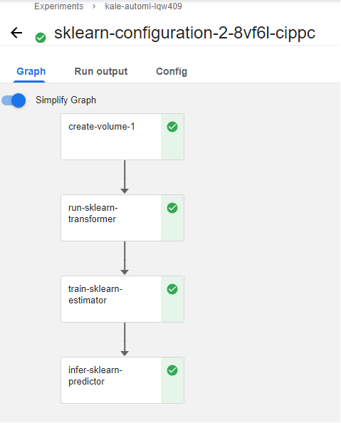
As you can see, the pipeline consists of an run-sklearn-transformer step that transforms the dataset, an train-sklearn-estimator step that trains the model, and an infer-sklearn-predictor step that predicts over the test dataset.
During the pipeline runs, Kale is logging MLMD artifacts in a persistent way. These artifacts are backed by Rok snapshots so they are versioned and persistent, regardless of the pipeline’s lifecycle. This way, you can have complete visibility of the inputs and outputs of the pipeline steps. And most importantly, you can always be aware of the dataset, the model, and the parameters used for the training process.
4. View the artifact of a Rok snapshot
If you click on the run-sklearn-transformer step, and you go to the ML Metadata tab, you can see the artifact of a Rok snapshot that contains the input dataset:
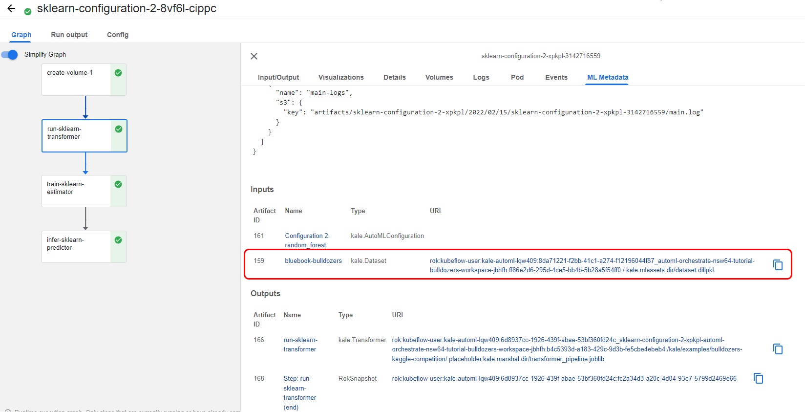
And a KaleTransformer, the object that is transforming the data:
![]()
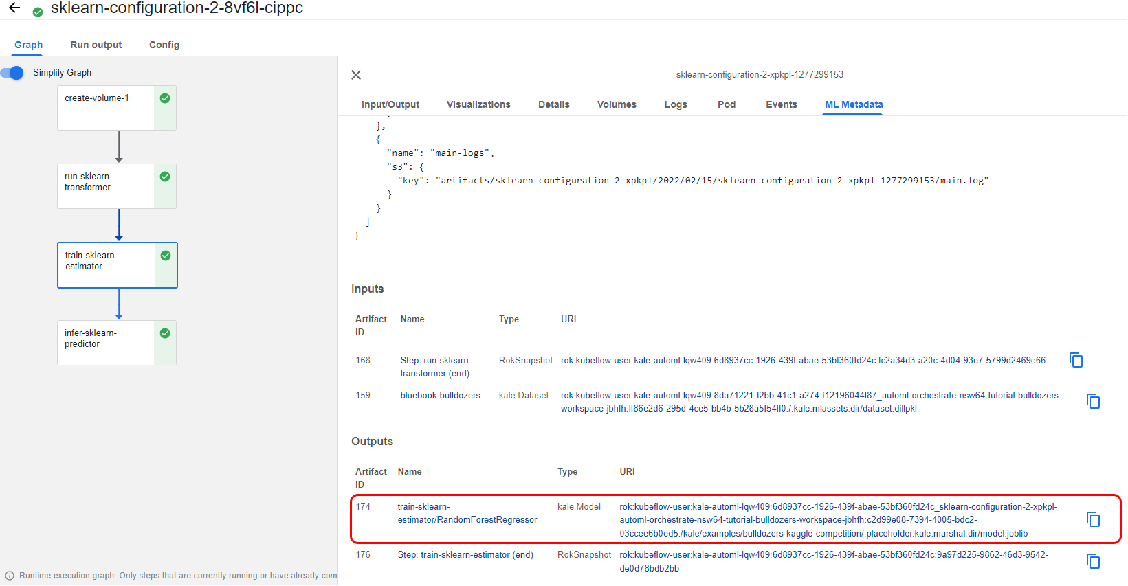
5. View the artifact of the trained model
If you go to the ML Metadata tab of the next step, called train-sklearn-estimator, you can see the artifact of the trained model:
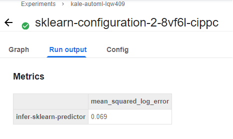
6. View the pipeline metrics
If you go to the Run output of this pipeline, you can view the pipeline Metrics. Here we have one, the mean squared logarithmic error. This metric shows you how well this particular auto-sklearn configuration performed on the dataset.
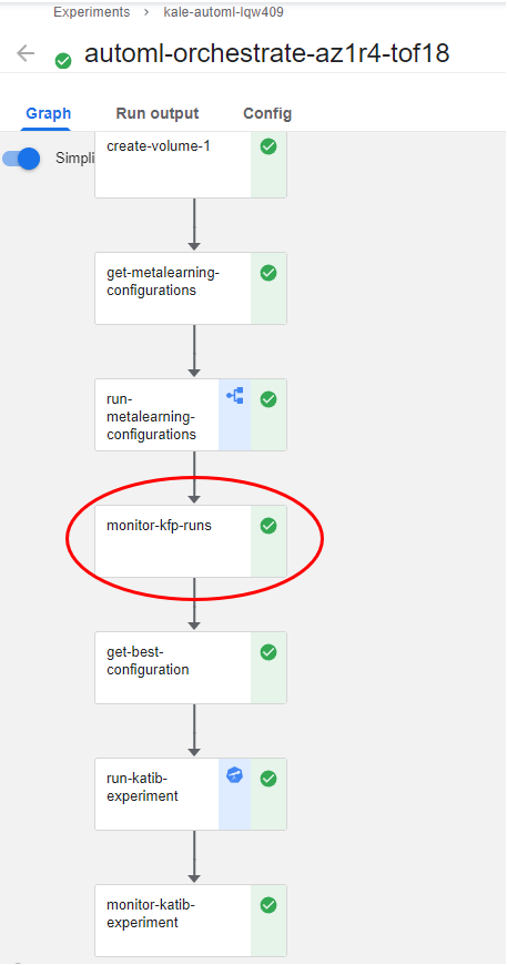
(Hands-On) Monitor the KFP Runs
Now, let’s go back to the orchestration pipeline and go through the next steps. The monitor-kfp-runs step waits for all the pipelines to complete, that is the four KFP runs that have different configurations.
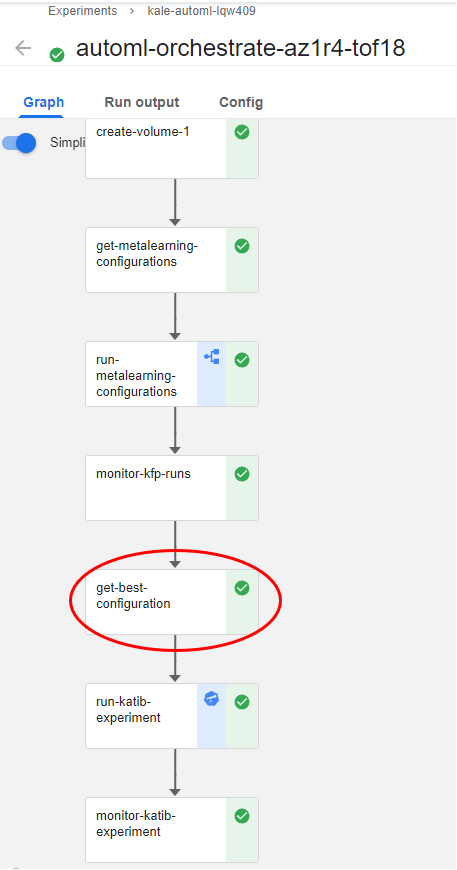
(Hands-On) Get the Best Configuration
When the runs succeed, Kale gets the one with the best performance. Kale knows, based on the optimization metric you provided in the notebook, if it needs to look for the highest or the lowest KFP metric value. This happens in the get-best-configuration step:
Hyperparameter Tuning w/ Katib Overview
Hyperparameter Tuning
Hyperparameter Tuning with Kubeflow’s AutoML component, Katib, optimizes machine learning models. Katib is agnostic to machine learning frameworks and performs hyperparameter tuning, early stopping, and neural architecture search written in various languages. Automated machine learning (AutoML) enables non-data science experts to make use of machine learning models and techniques and apply them to problems through automation. AutoML attempts to simplify
- Data pre-processing
- Feature engineering
- Feature extraction
- Feature selection
- Algorithm selection
- Hyperparameter tuning.
Hyperparameter Definition
| Values set beforehand | Values estimated during training with historical data |
|---|---|
| External to the model | Part of the model |
| Values are not saved as they are not part of the trained model | Estimated value is saved with the trained model |
| Independent of the dataset | Dependent on the dataset the system is trained with |
Tip: if you have to specify the value beforehand, it is a hyperparameter
- Example: A learning rate for training a neural network aka “early stopping”
- Example: The c and sigma hyperparameters for support vector machines.
- Example: The k in k-nearest neighbors.
Hyperparameter Tuning & Kale
You will continue to use Kale when working with Katib to orchestrate experiments so every Katib trial is a unique pipeline execution.
Kale has found the best configuration with the help of auto-sklearn. Note that this was a “Meta-Learning” suggestion, there is no reason to stop trying to further tune this model architecture. We want Kale to run a HP Tuning experiment, using Katib, to further explore different sets of initialization parameters, starting from the ones of this configuration. Kale will take care of creating a suitable search space, around these initialization parameters.
(Hands-On) Hyperparameter Optimization of the Model
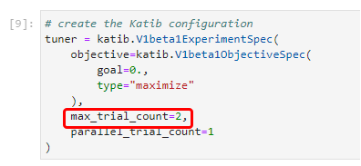
1. View the trials
You have already configured the Katib experiment in your notebook. As in the configuration case, the more trials you run the more chances you have to improve the original result. We expect to have no more than two trials as you can see in the code snippet below:
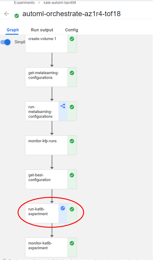
2. View the run-katib-experiment pipeline step
Notice that the run-katib-experiment pipeline step has the Katib logo as an icon. This means that in this step Kale produces a Katib experiment:
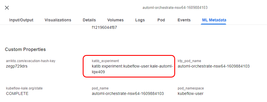
3. View the Katib experiment
If you click this step and go to the ML Metadata tab, you will find the link to the corresponding Katib experiment:
Click on the link to go to the Katib UI and view the experiment:
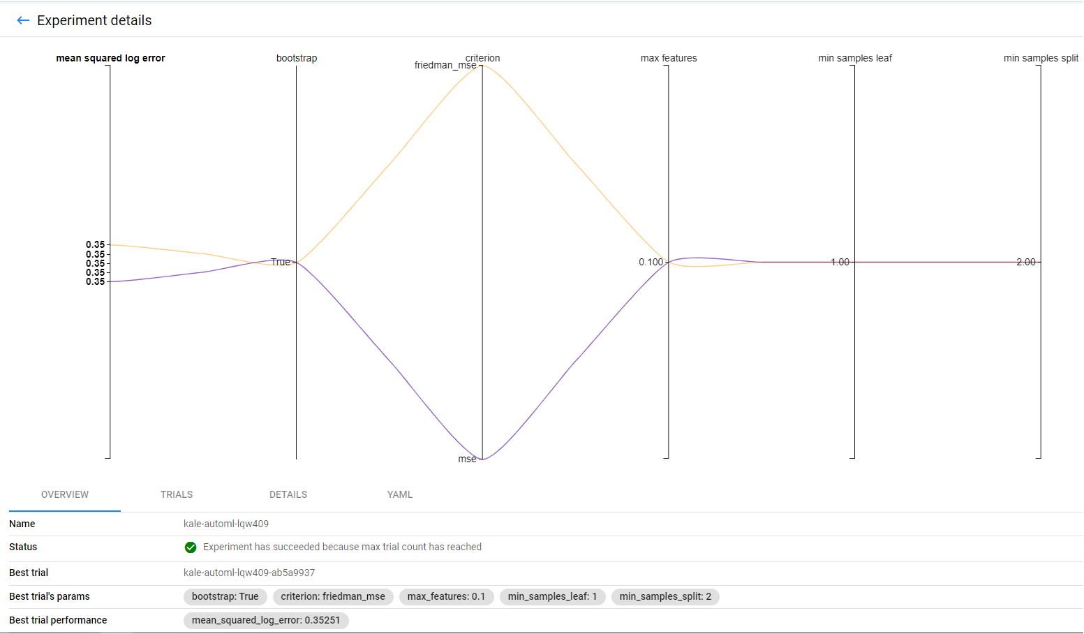
4. View the trials
Now, go to the TRIALS tab to view the two different trials and how they performed:
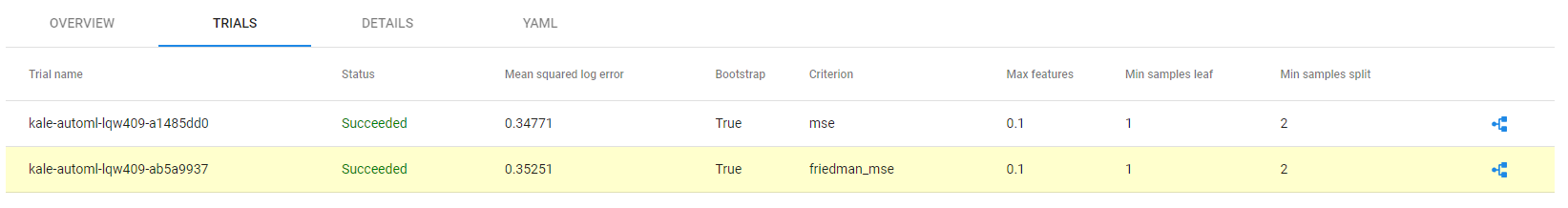
Notice that the best-performing trial is highlighted.
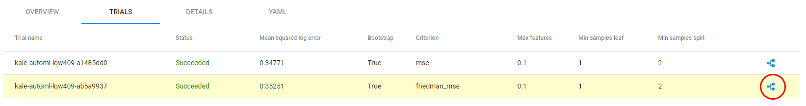
5. View the KFP run of the best Katib trial
Click on the pipeline icon on the right to view the KFP run that corresponds to this Katib trial:
Kale implements a shim to have the trials actually run pipelines in Kubeflow Pipelines, and then collect the metrics from the pipeline runs. This is the KFP run of the Katib trial that performed best:
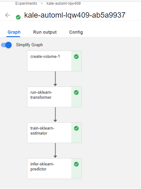
Notice that this pipeline is exactly the same as the configuration runs we described previously. This is expected, as we are running the same pipeline and changing the parameters to perform HP tuning. However, this KFP run has different run parameters from the configuration run.
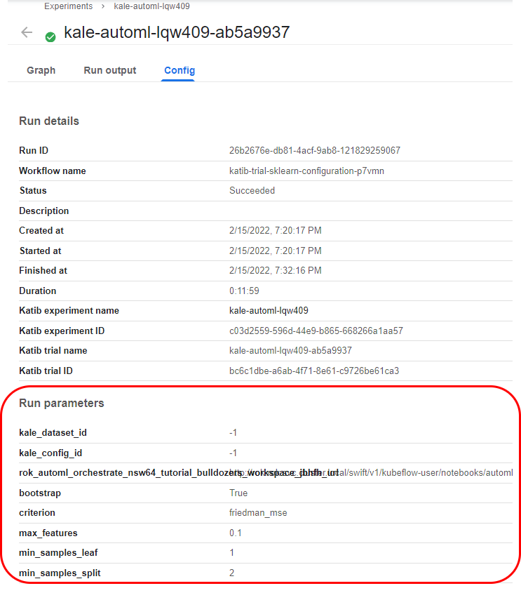
6. View the run parameters of the pipeline
If you go to the Config tab, you will see the run parameters of this pipeline. Katib was the one that selected these specific parameters.
Rok and the associated Rok Cluster sitting within the Kubeflow Cluster are responsible for taking, managing, securing, and sharing Kubeflow Pipeline Snapshots. Before proceeding please familiarize yourself with some of the benefits of Snapshotting that is made possible by Rok. By Combining Kale and Rok and the Multiple Read Write volumes in the Notebook Server, you can run multiple steps on multiple nodes, distribute the whole training and workload across the nodes, and maintain dependencies across these steps and nodes.