import numpy as np
import pandas as pd
import seaborn as sns
from matplotlib import pyplot as plt
from matplotlib import style

from sklearn import linear_model
from sklearn.linear_model import LogisticRegression
from sklearn.ensemble import RandomForestClassifier
from sklearn.linear_model import Perceptron
from sklearn.linear_model import SGDClassifier
from sklearn.tree import DecisionTreeClassifier
from sklearn.neighbors import KNeighborsClassifier
from sklearn.svm import SVC, LinearSVC
from sklearn.naive_bayes import GaussianNBMachine Learning on Titanic passengers survival data
This Notebook will use machine learning to create a model that predicts which passengers survived the Titanic shipwreck. The dataset provides information on the fate of passengers on the Titanic, summarized according to economic status (class), sex, age and survival.
Credit for this Notebook goes to Niklas Donges, who published a very detailed post here. Check it out if you want to dive deeper in the data analysis and machine learning details of the challenge.
Import dependencies and load data
path = "data/"

PREDICTION_LABEL = 'Survived'

test_df = pd.read_csv(path + "test.csv")
train_df = pd.read_csv(path + "train.csv")
Let’s explore the data
These are features of the dataset:
survival:    Survival
PassengerId: Unique Id of a passenger.
pclass:    Ticket class
sex:    Sex
Age:    Age in years
sibsp:    # of siblings / spouses aboard the Titanic
parch:    # of parents / children aboard the Titanic
ticket:    Ticket number
fare:    Passenger fare
cabin:    Cabin number
embarked: Port of Embarkationtrain_df.info()<class 'pandas.core.frame.DataFrame'>
RangeIndex: 891 entries, 0 to 890
Data columns (total 12 columns):
PassengerId 891 non-null int64
Survived 891 non-null int64
Pclass 891 non-null int64
Name 891 non-null object
Sex 891 non-null object
Age 714 non-null float64
SibSp 891 non-null int64
Parch 891 non-null int64
Ticket 891 non-null object
Fare 891 non-null float64
Cabin 204 non-null object
Embarked 889 non-null object
dtypes: float64(2), int64(5), object(5)
memory usage: 83.7+ KBtrain_df.describe()| PassengerId | Survived | Pclass | Age | SibSp | Parch | Fare | |
|---|---|---|---|---|---|---|---|
| count | 891.000000 | 891.000000 | 891.000000 | 714.000000 | 891.000000 | 891.000000 | 891.000000 |
| mean | 446.000000 | 0.383838 | 2.308642 | 29.699118 | 0.523008 | 0.381594 | 32.204208 |
| std | 257.353842 | 0.486592 | 0.836071 | 14.526497 | 1.102743 | 0.806057 | 49.693429 |
| min | 1.000000 | 0.000000 | 1.000000 | 0.420000 | 0.000000 | 0.000000 | 0.000000 |
| 25% | 223.500000 | 0.000000 | 2.000000 | 20.125000 | 0.000000 | 0.000000 | 7.910400 |
| 50% | 446.000000 | 0.000000 | 3.000000 | 28.000000 | 0.000000 | 0.000000 | 14.454200 |
| 75% | 668.500000 | 1.000000 | 3.000000 | 38.000000 | 1.000000 | 0.000000 | 31.000000 |
| max | 891.000000 | 1.000000 | 3.000000 | 80.000000 | 8.000000 | 6.000000 | 512.329200 |
train_df.head(8)| PassengerId | Survived | Pclass | Name | Sex | Age | SibSp | Parch | Ticket | Fare | Cabin | Embarked | |
|---|---|---|---|---|---|---|---|---|---|---|---|---|
| 0 | 1 | 0 | 3 | Braund, Mr. Owen Harris | male | 22.0 | 1 | 0 | A/5 21171 | 7.2500 | NaN | S |
| 1 | 2 | 1 | 1 | Cumings, Mrs. John Bradley (Florence Briggs Th... | female | 38.0 | 1 | 0 | PC 17599 | 71.2833 | C85 | C |
| 2 | 3 | 1 | 3 | Heikkinen, Miss. Laina | female | 26.0 | 0 | 0 | STON/O2. 3101282 | 7.9250 | NaN | S |
| 3 | 4 | 1 | 1 | Futrelle, Mrs. Jacques Heath (Lily May Peel) | female | 35.0 | 1 | 0 | 113803 | 53.1000 | C123 | S |
| 4 | 5 | 0 | 3 | Allen, Mr. William Henry | male | 35.0 | 0 | 0 | 373450 | 8.0500 | NaN | S |
| 5 | 6 | 0 | 3 | Moran, Mr. James | male | NaN | 0 | 0 | 330877 | 8.4583 | NaN | Q |
| 6 | 7 | 0 | 1 | McCarthy, Mr. Timothy J | male | 54.0 | 0 | 0 | 17463 | 51.8625 | E46 | S |
| 7 | 8 | 0 | 3 | Palsson, Master. Gosta Leonard | male | 2.0 | 3 | 1 | 349909 | 21.0750 | NaN | S |
Missing data
Let’s see here how much data is missing. We will have to fill the missing features later on.
total = train_df.isnull().sum().sort_values(ascending=False)
percent_1 = train_df.isnull().sum()/train_df.isnull().count()*100
percent_2 = (round(percent_1, 1)).sort_values(ascending=False)
missing_data = pd.concat([total, percent_2], axis=1, keys=['Total', '%'])
missing_data.head(5)| Total | % | |
|---|---|---|
| Cabin | 687 | 77.1 |
| Age | 177 | 19.9 |
| Embarked | 2 | 0.2 |
| Fare | 0 | 0.0 |
| Ticket | 0 | 0.0 |
Age and Sex
survived = 'survived'
not_survived = 'not survived'
fig, axes = plt.subplots(nrows=1, ncols=2,figsize=(10, 4))
women = train_df[train_df['Sex']=='female']
men = train_df[train_df['Sex']=='male']
ax = sns.distplot(women[women['Survived']==1].Age.dropna(), bins=18, label = survived, ax = axes[0], kde =False)
ax = sns.distplot(women[women['Survived']==0].Age.dropna(), bins=40, label = not_survived, ax = axes[0], kde =False)
ax.legend()
ax.set_title('Female')
ax.set_ylabel('Survival Probablity')
ax = sns.distplot(men[men['Survived']==1].Age.dropna(), bins=18, label = survived, ax = axes[1], kde = False)
ax = sns.distplot(men[men['Survived']==0].Age.dropna(), bins=40, label = not_survived, ax = axes[1], kde = False)
ax.legend()
ax.set_title('Male')
_ = ax.set_ylabel('Survival Probablity')
Embarked, Pclass and Sex
FacetGrid = sns.FacetGrid(train_df, row='Embarked', height=4.5, aspect=1.6)
FacetGrid.map(sns.pointplot, 'Pclass', 'Survived', 'Sex', palette=None,  order=None, hue_order=None )
_ = FacetGrid.add_legend()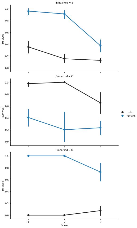
Pclass
Explore if Pclass is contributing to a person chance of survival
_ = sns.barplot(x='Pclass', y='Survived', data=train_df)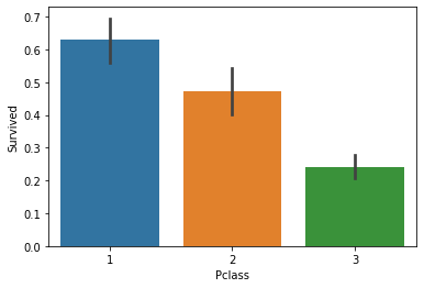
Here we confirm that being in class 1 increases the chances of survival, and that a person in class 3 has high chances of not surviving
grid = sns.FacetGrid(train_df, col='Survived', row='Pclass', height=2.2, aspect=1.6)
grid.map(plt.hist, 'Age', alpha=.5, bins=20)
grid.add_legend();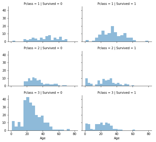
DATA PROCESSING
SibSp and Parch
Combine these two features as the number of relatives
data = [train_df, test_df]
for dataset in data:
    dataset['relatives'] = dataset['SibSp'] + dataset['Parch']
    dataset.loc[dataset['relatives'] > 0, 'not_alone'] = 0
    dataset.loc[dataset['relatives'] == 0, 'not_alone'] = 1
    dataset['not_alone'] = dataset['not_alone'].astype(int)
train_df['not_alone'].value_counts()
1 537
0 354
Name: not_alone, dtype: int64# Survival with respect to the number of relatives in the ship
axes = sns.catplot('relatives','Survived', kind='point',
data=train_df, aspect = 2.5, )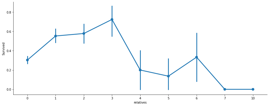
# This does not contribute to a person survival probability
train_df = train_df.drop(['PassengerId'], axis=1)
Missing data: Cabin
Create a new Deck feature
import re
deck = {"A": 1, "B": 2, "C": 3, "D": 4, "E": 5, "F": 6, "G": 7, "U": 8}
data = [train_df, test_df]

for dataset in data:
    dataset['Cabin'] = dataset['Cabin'].fillna("U0")
    dataset['Deck'] = dataset['Cabin'].map(lambda x: re.compile("([a-zA-Z]+)").search(x).group())
    dataset['Deck'] = dataset['Deck'].map(deck)
    dataset['Deck'] = dataset['Deck'].fillna(0)
    dataset['Deck'] = dataset['Deck'].astype(int)
# we can now drop the cabin feature
train_df = train_df.drop(['Cabin'], axis=1)
test_df = test_df.drop(['Cabin'], axis=1)
Missing data: Age
Fill missing data from age feature with a random sampling from the distribution of the existing values.
data = [train_df, test_df]

for dataset in data:
    mean = train_df["Age"].mean()
    std = test_df["Age"].std()
    is_null = dataset["Age"].isnull().sum()
    # compute random numbers between the mean, std and is_null
    rand_age = np.random.randint(mean - std, mean + std, size = is_null)
    # fill NaN values in Age column with random values generated
    age_slice = dataset["Age"].copy()
    age_slice[np.isnan(age_slice)] = rand_age
    dataset["Age"] = age_slice
    dataset["Age"] = train_df["Age"].astype(int)
train_df["Age"].isnull().sum()0Missing data: Embarked
train_df['Embarked'].describe()count 889
unique 3
top S
freq 644
Name: Embarked, dtype: object# fill with most common value
common_value = 'S'
data = [train_df, test_df]
for dataset in data:
dataset['Embarked'] = dataset['Embarked'].fillna(common_value)Convert Features
train_df.info()<class 'pandas.core.frame.DataFrame'>
RangeIndex: 891 entries, 0 to 890
Data columns (total 13 columns):
Survived 891 non-null int64
Pclass 891 non-null int64
Name 891 non-null object
Sex 891 non-null object
Age 891 non-null int64
SibSp 891 non-null int64
Parch 891 non-null int64
Ticket 891 non-null object
Fare 891 non-null float64
Embarked 891 non-null object
relatives 891 non-null int64
not_alone 891 non-null int64
Deck 891 non-null int64
dtypes: float64(1), int64(8), object(4)
memory usage: 90.6+ KBdata = [train_df, test_df]
for dataset in data:
dataset['Fare'] = dataset['Fare'].fillna(0)
dataset['Fare'] = dataset['Fare'].astype(int)Titles features
data = [train_df, test_df]
titles = {"Mr": 1, "Miss": 2, "Mrs": 3, "Master": 4, "Rare": 5}

for dataset in data:
    # extract titles
    dataset['Title'] = dataset.Name.str.extract(' ([A-Za-z]+)\.', expand=False)
    # replace titles with a more common title or as Rare
    dataset['Title'] = dataset['Title'].replace(['Lady', 'Countess','Capt', 'Col','Don', 'Dr',\
                                            'Major', 'Rev', 'Sir', 'Jonkheer', 'Dona'], 'Rare')
    dataset['Title'] = dataset['Title'].replace('Mlle', 'Miss')
    dataset['Title'] = dataset['Title'].replace('Ms', 'Miss')
    dataset['Title'] = dataset['Title'].replace('Mme', 'Mrs')
    # convert titles into numbers
    dataset['Title'] = dataset['Title'].map(titles)
    # filling NaN with 0, to get safe
    dataset['Title'] = dataset['Title'].fillna(0)
train_df = train_df.drop(['Name'], axis=1)
test_df = test_df.drop(['Name'], axis=1)
Sex into numeric
genders = {"male": 0, "female": 1}
data = [train_df, test_df]

for dataset in data:
    dataset['Sex'] = dataset['Sex'].map(genders)
Drop Ticket feature
train_df = train_df.drop(['Ticket'], axis=1)
test_df = test_df.drop(['Ticket'], axis=1)
Embarked into numeric
ports = {"S": 0, "C": 1, "Q": 2}
data = [train_df, test_df]

for dataset in data:
    dataset['Embarked'] = dataset['Embarked'].map(ports)
Age into categories
data = [train_df, test_df]
for dataset in data:
    dataset['Age'] = dataset['Age'].astype(int)
    dataset.loc[ dataset['Age'] <= 11, 'Age'] = 0
    dataset.loc[(dataset['Age'] > 11) & (dataset['Age'] <= 18), 'Age'] = 1
    dataset.loc[(dataset['Age'] > 18) & (dataset['Age'] <= 22), 'Age'] = 2
    dataset.loc[(dataset['Age'] > 22) & (dataset['Age'] <= 27), 'Age'] = 3
    dataset.loc[(dataset['Age'] > 27) & (dataset['Age'] <= 33), 'Age'] = 4
    dataset.loc[(dataset['Age'] > 33) & (dataset['Age'] <= 40), 'Age'] = 5
    dataset.loc[(dataset['Age'] > 40) & (dataset['Age'] <= 66), 'Age'] = 6
    dataset.loc[ dataset['Age'] > 66, 'Age'] = 6

# let's see how it's distributed train_df['Age'].value_counts()
Fare into categories
data = [train_df, test_df]

for dataset in data:
    dataset.loc[ dataset['Fare'] <= 7.91, 'Fare'] = 0
    dataset.loc[(dataset['Fare'] > 7.91) & (dataset['Fare'] <= 14.454), 'Fare'] = 1
    dataset.loc[(dataset['Fare'] > 14.454) & (dataset['Fare'] <= 31), 'Fare']   = 2
    dataset.loc[(dataset['Fare'] > 31) & (dataset['Fare'] <= 99), 'Fare']   = 3
    dataset.loc[(dataset['Fare'] > 99) & (dataset['Fare'] <= 250), 'Fare']   = 4
    dataset.loc[ dataset['Fare'] > 250, 'Fare'] = 5
    dataset['Fare'] = dataset['Fare'].astype(int)
New Features
Age times Class
data = [train_df, test_df]
for dataset in data:
    dataset['Age_Class']= dataset['Age']* dataset['Pclass']
Fare per person
for dataset in data:
    dataset['Fare_Per_Person'] = dataset['Fare']/(dataset['relatives']+1)
    dataset['Fare_Per_Person'] = dataset['Fare_Per_Person'].astype(int)
# Let's take a last look at the training set, before we start training the models.
train_df.head(10)| Survived | Pclass | Sex | Age | SibSp | Parch | Fare | Embarked | relatives | not_alone | Deck | Title | Age_Class | Fare_Per_Person | |
|---|---|---|---|---|---|---|---|---|---|---|---|---|---|---|
| 0 | 0 | 3 | 0 | 2 | 1 | 0 | 0 | 0 | 1 | 0 | 8 | 1 | 6 | 0 |
| 1 | 1 | 1 | 1 | 5 | 1 | 0 | 3 | 1 | 1 | 0 | 3 | 3 | 5 | 1 |
| 2 | 1 | 3 | 1 | 3 | 0 | 0 | 0 | 0 | 0 | 1 | 8 | 2 | 9 | 0 |
| 3 | 1 | 1 | 1 | 5 | 1 | 0 | 3 | 0 | 1 | 0 | 3 | 3 | 5 | 1 |
| 4 | 0 | 3 | 0 | 5 | 0 | 0 | 1 | 0 | 0 | 1 | 8 | 1 | 15 | 1 |
| 5 | 0 | 3 | 0 | 1 | 0 | 0 | 1 | 2 | 0 | 1 | 8 | 1 | 3 | 1 |
| 6 | 0 | 1 | 0 | 6 | 0 | 0 | 3 | 0 | 0 | 1 | 5 | 1 | 6 | 3 |
| 7 | 0 | 3 | 0 | 0 | 3 | 1 | 2 | 0 | 4 | 0 | 8 | 4 | 0 | 0 |
| 8 | 1 | 3 | 1 | 3 | 0 | 2 | 1 | 0 | 2 | 0 | 8 | 3 | 9 | 0 |
| 9 | 1 | 2 | 1 | 1 | 1 | 0 | 2 | 1 | 1 | 0 | 8 | 3 | 2 | 1 |
ML
Because the dataset does not provide labels for their testing-set, we need to use the predictions on the training set to compare the algorithms with each other
train_labels = train_df[PREDICTION_LABEL]Random Forest
random_forest = RandomForestClassifier(n_estimators=100)
random_forest.fit(train_df, train_labels)
acc_random_forest = round(random_forest.score(train_df, train_labels) * 100, 2)
Logistic Regression
logreg = LogisticRegression(solver='liblinear')
logreg.fit(train_df, train_labels)
acc_log = round(logreg.score(train_df, train_labels) * 100, 2)
Gaussian Naive Bayes
gaussian = GaussianNB()
gaussian.fit(train_df, train_labels)
acc_gaussian = round(gaussian.score(train_df, train_labels) * 100, 2)
Linear SVM
linear_svc = LinearSVC()
linear_svc.fit(train_df, train_labels)
acc_linear_svc = round(linear_svc.score(train_df, train_labels) * 100, 2)
/Users/StefanoFiora/.pyenv/versions/3.6.8/envs/kale-test/lib/python3.6/site-packages/sklearn/svm/base.py:931: ConvergenceWarning: Liblinear failed to converge, increase the number of iterations.
"the number of iterations.", ConvergenceWarning)Decision Tree
decision_tree = DecisionTreeClassifier()
decision_tree.fit(train_df, train_labels)
acc_decision_tree = round(decision_tree.score(train_df, train_labels) * 100, 2)
Results
results = pd.DataFrame({
    'Model': ['Support Vector Machines', 'logistic Regression',
              'Random Forest', 'Naive Bayes', 'Decision Tree'],
    'Score': [acc_linear_svc, acc_log,
              acc_random_forest, acc_gaussian, acc_decision_tree]})
result_df = results.sort_values(by='Score', ascending=False)
result_df = result_df.set_index('Score')
print(result_df)