OpenVaccine: COVID-19 mRNA Vaccine Degradation Prediction

In this Kaggle competition we try to develop models and design rules for RNA degradation. As the overview of the competition states:

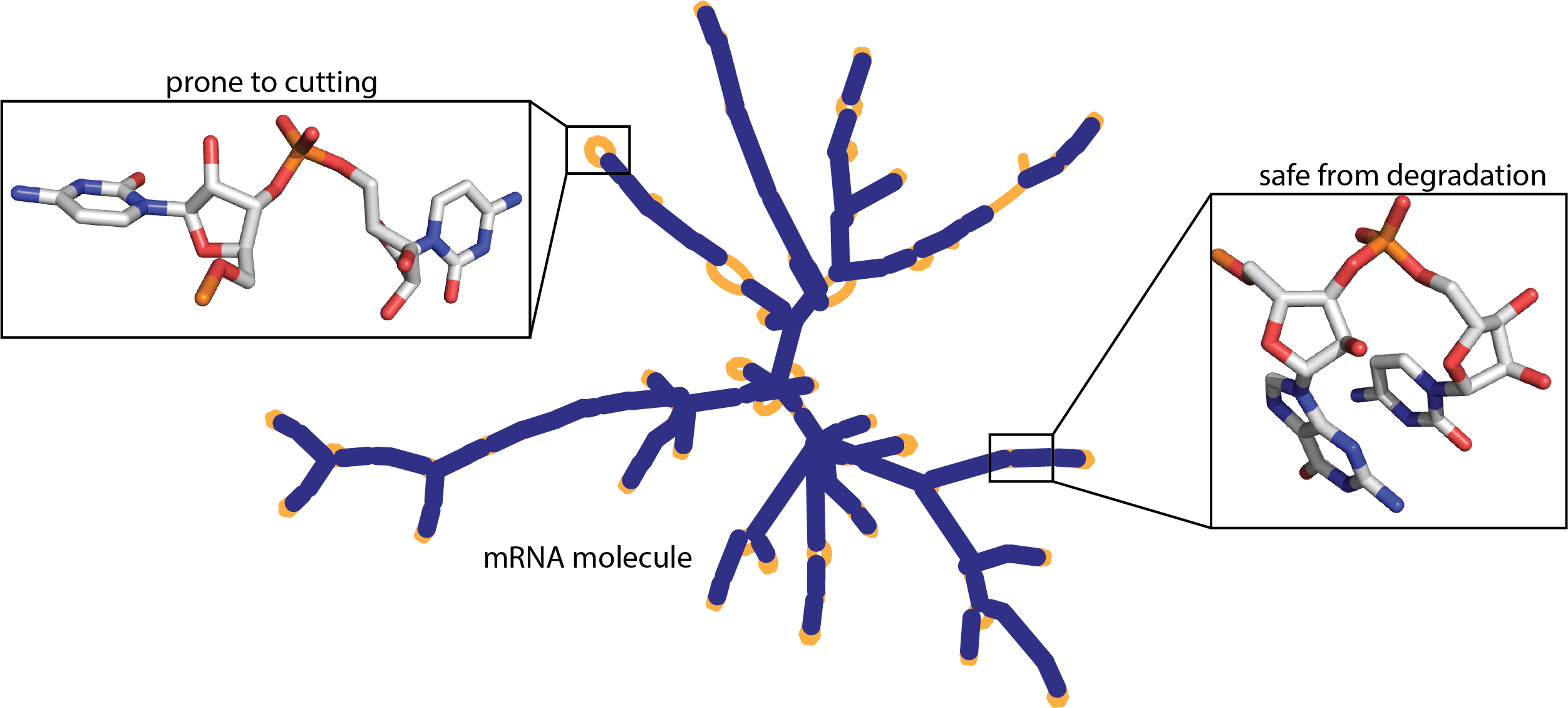
mRNA vaccines have taken the lead as the fastest vaccine candidates for COVID-19, but currently, they face key potential limitations. One of the biggest challenges right now is how to design super stable messenger RNA molecules (mRNA). Conventional vaccines (like your seasonal flu shots) are packaged in disposable syringes and shipped under refrigeration around the world, but that is not currently possible for mRNA vaccines.

Researchers have observed that RNA molecules have the tendency to spontaneously degrade. This is a serious limitation–a single cut can render the mRNA vaccine useless. Currently, little is known on the details of where in the backbone of a given RNA is most prone to being affected. Without this knowledge, current mRNA vaccines against COVID-19 must be prepared and shipped under intense refrigeration, and are unlikely to reach more than a tiny fraction of human beings on the planet unless they can be stabilized.

The model should predict likely degradation rates at each base of an RNA molecule. The training data set is comprised of over 3000 RNA molecules and their degradation rates at each position.

Install necessary packages

We can install the necessary package by either running pip install --user <package_name> or include everything in a requirements.txt file and run pip install --user -r requirements.txt. We have put the dependencies in a requirements.txt file so we will use the former method.

NOTE: Do not forget to use the --user argument. It is necessary if you want to use Kale to transform this notebook into a Kubeflow pipeline

!pip install --user -r requirements.txt

Imports

In this section we import the packages we need for this example. Make it a habit to gather your imports in a single place. It will make your life easier if you are going to transform this notebook into a Kubeflow pipeline using Kale.

import json
import numpy as np
import pandas as pd
import tensorflow as tf

from tensorflow.keras.preprocessing.text import Tokenizer

Project hyper-parameters

In this cell, we define the different hyper-parameters. Defining them in one place makes it easier to experiment with their values and also facilitates the execution of HP Tuning experiments using Kale and Katib.

# Hyper-parameters
LR = 1e-3
EPOCHS = 10
BATCH_SIZE = 64
EMBED_DIM = 100
HIDDEN_DIM = 128
DROPOUT = .5
SP_DROPOUT = .3
TRAIN_SEQUENCE_LENGTH = 107

Set random seed for reproducibility and ignore warning messages.

tf.random.set_seed(42)
np.random.seed(42)

tf.compat.v1.logging.set_verbosity(tf.compat.v1.logging.INFO)

Load and preprocess data

In this section, we load and process the dataset to get it in a ready-to-use form by the model. First, let us load and analyze the data.

Load data

The data are in json format, thus, we use the handy read_json pandas method. There is one train data set and two test sets (one public and one private).

train_df = pd.read_json("data/train.json", lines=True)
test_df = pd.read_json("data/test.json", lines=True)

We also load the sample_submission.csv file, which will prove handy when we will be creating our submission to the competition.

sample_submission_df = pd.read_csv("data/sample_submission.csv")

Let us now explore the data, their dimensions and what each column mean. To this end, we use the pandas head method to visualize a small sample (five rows by default) of our data set.

train_df.head()

We see a lot of strange entries, so, let us try to see what they are:

• sequence: An 107 characters long string in Train and Public Test (130 in Private Test), which describes the RNA sequence, a combination of A, G, U, and C for each sample.
• structure: An 107 characters long string in Train and Public Test (130 in Private Test), which is a combination of (, ), and . characters that describe whether a base is estimated to be paired or unpaired. Paired bases are denoted by opening and closing parentheses (e.g. (….) means that base 0 is paired to base 5, and bases 1-4 are unpaired).
• predicted_loop_type: An 107 characters long string, which describes the structural context (also referred to as ‘loop type’) of each character in sequence. Loop types assigned by bpRNA from Vienna RNAfold 2 structure. From the bpRNA_documentation: S: paired “Stem” M: Multiloop I: Internal loop B: Bulge H: Hairpin loop E: dangling End X: eXternal loop.

Then, we have signal_to_noise, which is quality control feature. It records the measurements relative to their errors; the higher value the more confident measurements are.

The *_error_* columns calculate the errors in experimental values obtained in corresponding reactivity and deg_* columns.

The last five columns (i.e., recreativity and deg_*) are out depended variables, our targets. Thus, for every base in the molecule we should predict five different values.

These are the main columns we care about. For more details, visit the competition info.

Preprocess data

We are now ready to preprocess the data set. First, we define the symbols that encode certain features (e.g. the base symbol or the structure), the features and the target variables.

symbols = "().ACGUBEHIMSX"
feat_cols = ["sequence", "structure", "predicted_loop_type"]
target_cols = ["reactivity", "deg_Mg_pH10", "deg_Mg_50C", "deg_pH10", "deg_50C"]
error_cols = ["reactivity_error", "deg_error_Mg_pH10", "deg_error_Mg_50C", "deg_error_pH10", "deg_error_50C"]

In order to encode values like strings or characters and feed them to the neural network, we need to tokenize them. The Tokenizer class will assign a number to each character.

tokenizer = Tokenizer(char_level=True, filters="")
tokenizer.fit_on_texts(symbols)

Moreover, the tokenizer keeps a dictionary, word_index, from which we can get the number of elements in our vocabulary. In this case, we only have a few elements, but if our dataset was a whole book, that function would be handy.

NOTE: We should add 1 to the length of the word_index dictionary to get the correct number of elements.

# get the number of elements in the vocabulary
vocab_size = len(tokenizer.word_index) + 1

We are now ready to process our features. First, we transform each character sequence (i.e., sequence, structure, predicted_loop_type) into number sequences and concatenate them together. The resulting shape should be (num_examples, 107, 3).

Now, we should do this in a way that would permit us to use this processing function with KFServing. Thus, since Numpy arrays are not JSON serializable, this function should accept and return pure Python lists.

def process_features(example):
    import numpy as np

    sequence_sentences = example[0]
    structure_sentences = example[1]
    loop_sentences = example[2]
    
    # transform character sequences into number sequences
    sequence_tokens = np.array(
        tokenizer.texts_to_sequences(sequence_sentences))
    structure_tokens = np.array(
        tokenizer.texts_to_sequences(structure_sentences))
    loop_tokens = np.array(
        tokenizer.texts_to_sequences(loop_sentences))
    
    # concatenate the tokenized sequences
    sequences = np.stack(
        (sequence_tokens, structure_tokens, loop_tokens),
        axis=1)
    sequences = np.transpose(sequences, (2, 0, 1))
   
    prepared = sequences.tolist()
    return prepared[0]

In the same way we process the labels. We should just extract them and transform them into the correct shape. The resulting shape should be (num_examples, 68, 5).

def process_labels(df):
    df = df.copy()
    
    labels = np.array(df[target_cols].values.tolist())
    labels = np.transpose(labels, (0, 2, 1))
    
    return labels

public_test_df = test_df.query("seq_length == 107")
private_test_df = test_df.query("seq_length == 130")

We are now ready to process the data set and make the features ready to be consumed by the model.

x_train = [process_features(row.tolist()) for _, row in train_df[feat_cols].iterrows()]
y_train = process_labels(train_df)

unprocessed_x_public_test = [row.tolist() for _, row in public_test_df[feat_cols].iterrows()]
unprocessed_x_private_test = [row.tolist() for _, row in private_test_df[feat_cols].iterrows()]

Define and train the model

We are now ready to define our model. We have to do with sequences, thus, it makes sense to use RNNs. More specifically, we will use bidirectional Gated Recurrent Units (GRUs) and Long Short Term Memory cells (LSTM). The output layer shoud produce 5 numbers, so we can see this as a regression problem.

First let us define two helper functions for GRUs and LSTMs and then, define the body of the full model.

def gru_layer(hidden_dim, dropout):
    return tf.keras.layers.Bidirectional(
         tf.keras.layers.GRU(hidden_dim, dropout=dropout, return_sequences=True, kernel_initializer = 'orthogonal')
    )

def lstm_layer(hidden_dim, dropout):
    return tf.keras.layers.Bidirectional(
        tf.keras.layers.LSTM(hidden_dim, dropout=dropout, return_sequences=True, kernel_initializer = 'orthogonal')
    )

The model has an embedding layer. The embedding layer projects the tokenized categorical input into a high-dimensional latent space. For this example we treat the dimensionality of the embedding space as a hyper-parameter that we can use to fine-tune the model.

def build_model(vocab_size, seq_length=int(TRAIN_SEQUENCE_LENGTH), pred_len=68,
                embed_dim=int(EMBED_DIM),
                hidden_dim=int(HIDDEN_DIM), dropout=float(DROPOUT), sp_dropout=float(SP_DROPOUT)):
    inputs = tf.keras.layers.Input(shape=(seq_length, 3))

    embed = tf.keras.layers.Embedding(input_dim=vocab_size, output_dim=embed_dim)(inputs)
    
    reshaped = tf.reshape(
        embed, shape=(-1, embed.shape[1],  embed.shape[2] * embed.shape[3])
    )
    
    hidden = tf.keras.layers.SpatialDropout1D(sp_dropout)(reshaped)
    
    hidden = gru_layer(hidden_dim, dropout)(hidden)
    hidden = lstm_layer(hidden_dim, dropout)(hidden)
    
    truncated = hidden[:, :pred_len]
    
    out = tf.keras.layers.Dense(5, activation="linear")(truncated)
    
    model = tf.keras.Model(inputs=inputs, outputs=out)
    
    return model

model = build_model(vocab_size)

model.summary()

Submissions are scored using MCRMSE (mean columnwise root mean squared error):

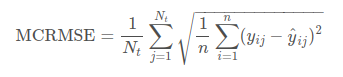
Thus, we should code this metric and use it as our objective (loss) function.

class MeanColumnwiseRMSE(tf.keras.losses.Loss):
    def __init__(self, name='MeanColumnwiseRMSE'):
        super().__init__(name=name)

    def call(self, y_true, y_pred):
        colwise_mse = tf.reduce_mean(tf.square(y_true - y_pred), axis=1)
        return tf.reduce_mean(tf.sqrt(colwise_mse), axis=1)

We are now ready to compile and fit the model.

model.compile(tf.optimizers.Adam(learning_rate=float(LR)), loss=MeanColumnwiseRMSE())

history = model.fit(np.array(x_train), np.array(y_train), 
                    validation_split=.1, batch_size=int(BATCH_SIZE), epochs=int(EPOCHS))

validation_loss = history.history.get("val_loss")[0]

Evaluate the model

Finally, we are ready to evaluate the model using the two test sets.

model_public = build_model(vocab_size, seq_length=107, pred_len=107)
model_private = build_model(vocab_size, seq_length=130, pred_len=130)

model_public.set_weights(model.get_weights())
model_private.set_weights(model.get_weights())

public_preds = model_public.predict(np.array([process_features(x) for x in unprocessed_x_public_test]))
private_preds = model_private.predict(np.array([process_features(x) for x in unprocessed_x_private_test]))

Serve the Model

We can leverage the Kale serve package to create an InferenceService. This way, we can easily deploy our model to Kubeflow and serve it as a REST API.

The first step is to create a preprocess function that will be used to create a transformer component for our InferenceService. This function should take the raw data as input and return the preprocessed data.

def preprocess(inputs):
    res = list()
    for instance in inputs["instances"]:
        res.append(process_features(instance))
    return {**inputs, "instances": res}

Finally, we can use the serve function provided by Kale to create an InferenceService. This function takes the model, the preprocess function and a configuration object as input.

from kale.common.serveutils import serve

config  = {"limits": {"memory": "4Gi"}}

server = serve(model, preprocessing_fn=preprocess,
               preprocessing_assets={"process_features": process_features,
                                     "tokenizer": tokenizer},
               deploy_config=config)

Invoke the InferenceService to get back the predictions.

data = json.dumps({"instances": unprocessed_x_public_test})
predictions = server.predict(data)
predictions

Submission

Last but note least, we create our submission to the Kaggle competition. The submission is just a csv file with the specified columns.

preds_ls = []

for df, preds in [(public_test_df, public_preds), (private_test_df, private_preds)]:
    for i, uid in enumerate(df.id):
        single_pred = preds[i]

        single_df = pd.DataFrame(single_pred, columns=target_cols)
        single_df['id_seqpos'] = [f'{uid}_{x}' for x in range(single_df.shape[0])]

        preds_ls.append(single_df)

preds_df = pd.concat(preds_ls)
preds_df.head()

submission = sample_submission_df[['id_seqpos']].merge(preds_df, on=['id_seqpos'])
submission.to_csv('submission.csv', index=False)